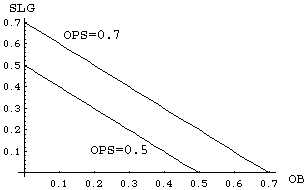
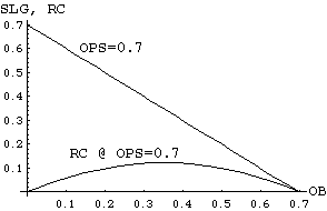
A simple plot will make the problems with OPS clear. Players whose OPS is a constant are (supposedly) indistingushable from one another, so it is instructive to examine what this means quantitatively. If we plot OB on the vertical axes and SLG on the horizontal axis, then players of equal OPS will lie along lines of slope -1 in the plane:
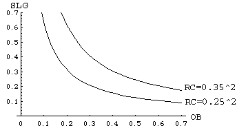
On the other hand, players with equal RC (per plate appearence or OB*SLG) form a hyperbola in the (OB,SLG) plane.
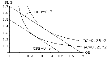
It is clear from these plots that only when OB and SLG are very close (that is, OB is roughly equal to SLG) does OPS approximate RC well:
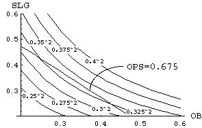
Another way to compare the two measures is to plot what a constant OPS contour looks like when it is mapped into the RC formula. To do this we simply take the formula for a constant OPS contour (SLG= -OB+c) and substitute it into f=OB*SLG. This gives g=OB*(c-OB) where c is the OPS value of interest.
This plot makes it clear that OPS is mapping players of dissimilar RC value into the same class, a potentially dangerous result when one is interested in ranking player ability for trades or drafts. This phenomenon can easily occur in the typical range of player abilities, as the next plot will make clear.
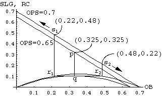
Here we have plotted the OPS to RC contour mapping for OPS=0.65 and OPS=0.7. A player at (OB,SLG) of (0.325,0.325) on the OPS=0.65 contour is actually superior to all players with OB<0.22 or OB>0.48 on the OPS=0.7 contour. This is shown graphically via the following procedure. Draw a vertical line from a point p on OPS=0.65 contour down to it’s corresponding point q on the RC mapping curve. [In this case we have chosen p=(0.325,0.325) on the OPS=0.65 contour.] Then draw a horizontal line thru point q and find the 2 intersection points r1 and r2 with the OPS=0.7 RC mapping curve. Then verticle lines from r1 and r2 up to the corresponding OPS=0.7 contour give you the points s1 and s2 on the OPS=0.7 contour that are ‘equvalent’ to point p in terms of RC value.
The closer we make the two OPS contours, the poorer OPS does in terms of correctly sorting out the ‘true’ (in terms of RC) differences between players. For example, a player at (0.3,0.3) with OPS=0.6 is actually better than all players of OPS=0.605 with OB<0.264 and OB>0.341, and he is better than all players of OPS=0.601 with OB<0.283 and OB>0.318. In essence, OPS overrates low OB, high SLG and hi OB, low SLG players. As there are generally many low OB, high SLG players in a given card set (particularly given the super advanced ballpark homerun rules), OPS can easily cause one to overrate such players to the detriment of one’s overall team quality. If one is playing in a high ballpark homerun stadium, OPS could cause a significant and costly (in terms of winning %) skew towards low OB sluggers in player selection.
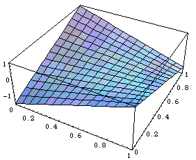
In order to make the errors inherent in OPS as explicit as possible, consider the following two figures. Figure 6 is a plot of 'whitened' OPS minus 'whitened' RC. Positive values indicate regions in the (OB,SLG) plane where OPS overestimates relative value with respect to RC, and negative values are regions where OPS underestimates relative value. Since OPS and RC have intrinsically different scales, Figure 6 was generated by mapping both OPS and RC to have an average value of 0 and a variance of 1.0 over the unit square (this is what 'whitening' essentially means for the purposes of this discussion). This makes the two measures directly comparable in a statistical sense. Since OPS is trying to estimate RC, one can then see how good that estimation is by taking the difference of the two whitened functions.
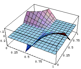
To make regions of over- and under-prediction clearer, Figure 7 is a repeat of Figure 6 with a flat surface at height 0 (i.e., the level at which whitened OPS and RC coincide) included:
In summary, be very careful when using OPS to approximate RC - you may not like what you get !!!!